JIT

Recreational music making means that you're constantly on the lookout for new sounds and samples that spark your creativity. This is what turned me towards audio source separation, wanting to use the same types of samples that I heard in the songs I love. One open-source model that does this is HDemucs, which separates a song into the categories "vocals", "drums", "bass", and "other". Take for example this snippet from Raye's "Worth It":

Which is separated into:

The model is essentially trying to revert information loss from when the individual audio sources were added together, since we don't know where each individual frequency of audio came from. This is a hard problem and the model is not perfect. You can for example hear some of the guitar's reverb in the vocal track.

I ran the model using PyTorch on my laptop. But then I fell into the timeless trap of thinking "I wonder if I can make it run faster?" since I then can churn out shitty music way faster.

The following details getting a grasp of JIT-compilation, rewriting a PyTorch audio source separation model in JAX to achieve a ~3x speedup, and optimizing its round-trip runtime on Modal by 10x.

maybe I can

Let's just first establish a benchmark. Running the model on audio files of different lengths on my macbook yields about a 0.32 real-time factor (RTF). Note here also that before each measurement we did a warmup run on the audio file to trigger compilation - as to not include compilation time in the "inference speed" measurement.

An RTF of 0.32 means that the model runs in about a third of the time of the audio file it's processing. So for example a 180s file would take about 60s.

How do we speed this up? Just-in-time compilation is a concept that has been around for a while, but has become more widely adopted in most ml libraries. Roughly: can we look at the graph of operations materialized at inference time, and optimize it just as the first forward pass is done?

In PyTorch you simply do torch.compile(model). How much speedup do we get from this?

Barely anything!

paying off some comprehension debt

Ok wait what is torch.compile actually doing here? Before figuring out why it didnt help, lets back up to what compilation is even trying to do. My mental model here says that the forward function of the model is flagged for compilation, but the compilation doesnt happen just yet. It happens when we actually run the model: just in time. This is because we need to know what the computational graph looks like, which is dependent on what input the model is called with.

The idea is to then look at this graph - in turn made up of the mathematical operations that define the model: matrix multiplications, exponentials, etc - and make it take less time to execute on hardware. The mathematical operations are performed using kernels (the most ambiguous name in math & computer science imo), implementations of mathematical operations in code, eg cuda. So one kernel might be some CUDA code that performs matrix multiplication.

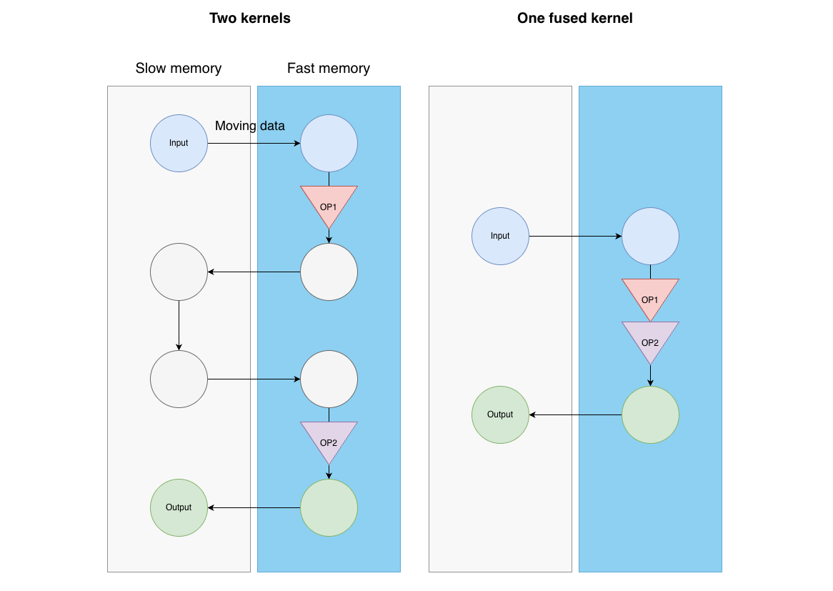
So what inefficiencies are typical? Whenever we need to launch a kernel on a GPU, we need to move data from slow memory (HBM) to fast memory (SRAM), perform our calculations, and then move the results back to slow memory. And with most AI-models being famously memory bound, that is the kernel usually has to sit waiting for more data to arrive to perform computations on because moving data is so slow. So we ideally want to minimize the number of times we move data to and from fast memory. One example is finding two operations that are done sequentially using their own kernels, and replacing them with a single kernel. For example, matrix multiplication, and exponentiation. If we write a single kernel for doing both of these ops while the data is on the fast memory, we can eliminate one back / forth data shuffle! This is typically called operator fusion. A rough mental model:

Okay so when we're doing torch.compile we fuse some kernels etc and make things fast. But why aren't we seeing that much of a speedup? That has to do with the computational graph of the HDemucs model, i.e. how it was written.

Torch compilation is written in a way so that it's easy to use, and falls back to regular eager execution when jit compilation doesnt work. So why isn't it working?

Again, performing jit compilation involves tracing an input through the model's compute graph to identify potential optimizations. This means that the compute graph we obtain and the one we optimize is directly tied to the first input we received / gave at compile time. A challenge arises in the case that a new input results in a new code path in the function. We here hit code that we havent optimized, and in turn trigger "recompilation". Imagine having a function which has a different code path for each input it receives. This means we'd have to recompile and optimize the compute graph for every new input, making it very inefficient. It also goes against the whole idea of compilation here - having a predictable compute graph known ahead of time that we can be smart about, since we know exactly which path the next data will take. Looking at the HDemucs code, we see that it actually has several places where the code branches based on the input, e.g. its shape:

# In _HEncLayer.forward() - Line 153
if not self.freq and x.dim() == 4:
    B, C, Fr, T = x.shape
    x = x.view(B, -1, T)

This means that input with x.dim() != 4 takes one path, and x.dim() == 4 another, triggering recompilation. And we can actually see this when we run the forward pass of the compiled model:

[3/8] torch._dynamo hit config.recompile_limit (8)
   function: 'forward' (/torchaudio/models/_hdemucs.py:136)
   last reason: 3/7: tensor 'x' rank mismatch. expected 4, actual 3

Here torch.compile has a recompile limit of 8, meaning that it gives up compiling more than 8 different graph variants. And here we see that it hit another recompile when we had compiled for x.dim() == 4, but it came in with x.dim() == 3.

There is of course nothing wrong with this code - its written with modularity and re-usability in mind. But this is what we have to trade off for speed when using jit compilation - predictability. This is the first challenge of jit compilation - that the actual code path might deviate from the one we compiled for.

So okay, the original implementation of the model wasnt written with jit compilation in mind. What can we do about that?

Rewriting it in JAX

So I rewrote the model's ~1000 lines in JAX. JAX is a numerical computing library designed around composable function transformations - one of which is JIT compilation. And similarly it also has a library with common ML layers and components called FLAX.

Beyond predictable control flow, another aspect to consider to get the most out of compilation is pure functions. A pure function is a function that does not modify or cause any external side effects, such as updating a global variable. One reason pure functions are preferential for jit compilation is that their order can be rearranged while guaranteeing the same result. We can also cache them effectively since they always return the same result given the same input. With impure functions we cant guarantee we will get the same result if we reorder the functions since some external state could have been modified which the other function uses. To dive deeper into these concepts i recommend Common Gotchas in JAX.

The process involved rewriting each module of the HDemucs model from pytorch to flax, and then creating a numerical diff test based on some sample inputs / outputs to ensure the behaviour is matched numerically both for random and trained weights. For the trained weights I then had to parse the pytorch models weights, extract each tensor, and convert it into jax format. The whole "get exactly the same numerical behaviour" also proved to be a real headache sometimes. For example:

• Implementing interceptors / forward hooks both for the jax and pytorch model to be able to debug tensor shapes, dtypes, and norms
• Discovering non obvious differences between flax and pytorch modules, such as flax gelu using tanh approximation by default and not torch, flax using a different ordering for the conv layer shape ordering.
• and ofc rethinking the code to make it work with jit compilation

After having done this, the L2 norm diff of a forward pass on a dummy 180s audio file is 0.000497, and pretty much inaudible to me. Since the purpose here is only inference and not training, I decided to be satisfied with that.

So how does the speed compare then? I ran the vanilla flax and the jit compiled flax model on the same set of audio files.

• the JIT compiled flax version is the fastest as we expect!
• But interestingly the non-compiled flax implementation runs faster than the pytorch one out of the box. Why?

The interesting thing to note here is that JAX eager execution works by lowering each Python operation to HLO (high level optimizer) and compiled by the XLA compiler individually, then executed immediately. HLO is a framework independent representation of the compute graph, a little like an intermediate representation of the model inbetween the python code and the hardware-specific kernels. The HLO graph is what would be optimized by a jit compiler to achieve speedup, but we're not doing that yet. However, JAX still tries to be smart via a couple of things:

• Even compiled individually, each op still gets XLA-level optimizations like memory layout and vectorization - some initial overhead, but speedup for later ops.
• Caching of compiled operations. Once eg a convolution of a certain shape signature has been compiled and optimized, we save it, and since we perform operations with the same shape several times in the model, we can achieve a speedup

So JAX still does some tricks even when not explicitly jit compiling the model compute graph, and thats why its still faster than the vanilla pytorch one.

So what has the jit compiled flax model done to achieve even further speedups? Inspecting the compiled model reveals that it actually has done a bunch of kernel fusion. One such example that the XLA compiler did was for the forward pass of the LSTM cell, which includes the following ops:

Input: f32[1,192], f32[192]
  │
  ├─ constant(1.0)
  ├─ broadcast
  ├─ negate(x)           ─┐
  ├─ exp(-x)              │  sigmoid(x) = 1/(1+exp(-x))
  ├─ add(exp, 1)          │
  ├─ divide(1, sum)      ─┘
  ├─ bitcast
  ├─ tanh(other_input)
  └─ multiply(sigmoid, tanh)  →  Output: f32[1,192]

These were fused into a single kernel, making us avoid having to move data to and from memory between each call!

Okay so it runs pretty quickly on my macbook, achieving around a ~3x speedup over vanilla PyTorch. Can we achieve even bigger speedups?

GPU

ok lets now try running the model on a gpu on modal. I used an A100 80GB since we were hitting quite large memory reqs > 40 GB when running the longest audio file.

Some interesting things to note:

1. Regular flax is the slowest. My idea here is that without JIT, JAX compiles and launches a separate CUDA kernel for every operation. On GPU this per-op kernel launch overhead dominates, whereas on CPU the overhead is much smaller and the XLA-compiled individual ops still give a net benefit.
2. PyTorch vanilla and compiled are about equally fast. Similarly to the CPU case, the PyTorch implementation is not optimal for compilation, causing recompilation and fallback to eager mode due to eg dynamic control flows in the forward pass.
3. JIT compiled flax is the fastest. The advantage here is that we compile once for each audio length, and then use this optimized compute graph for each forward pass, which is what we're actually measuring. Note though that we're still incurring an initial compilation cost which is not included in the benchmark time. But the advantage over vanilla flax is that the XLA compiler optimizes the compute graph holistically, not just each op, allowing for more speedup!

Overall this means that we can run audio source separation of a typical 3m song (180s) in under a second - about a ~3.8x speedup over vanilla PyTorch on GPU.

Ultimately both torch and jax benefit from just running on better hardware here, with higher memory bandwidth and faster compute.

using the model irl

We've considered the isolated single file case where we're just running the model on a single audio file on a gpu. But that's not how we'd use it in the real world. In that case we'd want to:

• support a range of audio file lengths that users might supply
• be as fast as possible for all of these
• ideally fully utilize the gpu's compute and memory bandwidth to get our moneys worth.

The thing with jit compilation in this context is that we need to compile the model's forward pass for a certain input, ie for a certain length of audio we want to separate. If we then run it with another audio length we have to recompile it. And when using the model in an application this recompilation incurs latency for the user. One way to handle this is to compile the model for a specific input length, say 30s. And then if we want to separate an audio file of 60s, we just run it twice on two 30s windows. And further, since these computations are not dependent on eachother we can even run them in parallel. So when I wanted to expose this model to users that's what I did, which was originally detailed in the torchaudio blog post.

There are a couple of catches:

• How do we handle arbitrary audio file lengths? We pad until we hit a multiple of 30s (or whatever we compiled the model with)
• What if the audio file is larger than the gpu can handle memory-wise? The simple solution is to put an upper limit on how long audio files the user can upload. The more complicated one is to tune the separation algorithm to process the audio sequentially as to not hit the gpu memory limit and deliver results in chunks. I went for the first option.
• we also overlap the windows we separate and cross fade in order to avoid clicks / pops/ artifacts at transitions

for choosing the audio length to compile for it comes down to what lengths youll actually run the model on, ie the distribution of input lengths. This is something you'd ideally tune in a real application after observing the distribution of lengths of audio files that your users send in to the application. To not fall down this rabbit hole too much i just went with 30s.

deploying on modal

Beside the inference side, there are also several aspects to consider when actually deploying the model on a serverless platform like modal and serving real user requests:

• The user has to wait for the audio file to be uploaded
• Since Modal is scale to zero by default (which is nice to save costs) a potential first request has to wait for the container to cold start, and maybe even more importantly: wait for the initial jit compilation to finish
• Then inference happens
• And lastly we have to move the generated audio files from the server to the user

These are all practical deployment challenges. Some ideas to combat them include:

• caching the result of the jit compilation via the env var JAX_COMPILATION_CACHE_DIR - each new container doesn't have to re-compile the forward pass, instead it just reads it from eg disk
• minimizing the round trip distance for file upload / download via Modal tunnels. Modal containers are (by default) subject to be scheduled in many different cloud regions. Traffic to them also has to go through the modal control plane (us-east-1). This means any file to / from the user could potentially have to travel a long way. For example, with the code serving the frontend running in Stockholm, and the model running via modal in Frankfurt, the user file has to go from client -> stockholm -> us-east-1 -> frankfurt and then the same way back. A tunnel is here a way to provide a direct connection from the code in stockholm to the modal container running the model in Frankfurt, skipping a lot of travel time!
• keeping the container warm, which avoids the initial cold start latency for the user

I implemented a simple API for the model running on modal, and aimed to utilize these potential speedups. I ran a range of different payloads against it, and recorded how much time each phase of the request took using each type of speedup:

• We see that the baseline time is largely dominated by network overhead and model load + jit
• Caching the jit compiled model reduces total time by about ~50s
• Using a direct tunnel also significantly brings down the network time
• And lastly also keeping the container warm skips the cold start, bringing total round trip time to around 14s

Putting these together gets us the ~10x round trip improvement mentioned at the start.

epilogue

Approaches still left on the table:

• Running the model in fp16 to reduce both load times and inference time. The challenge here is that some of the flax conv layers do not support fp16, forcing constant conversion - ultimately not making fp16 worth it. But if resolved it could have a big impact
• Modal memory snapshotting - capturing the container's memory just before code starts to run, saving it, and loading via cache at next container startup. Explored this a bit, but since GPU memory snapshots are still in beta (and I encountered some hiccups with them) I skipped including it
• Tuning the rest of the code, eg maybe a better data format, pre- and post-inference processing, etc

Lastly: a real deployment with constant traffic would be a different beast, horizontal scaling, batching, and requiring tuning of things like the target compilation time based on user song input distribution, and considering dynamic jit re-compilation.