dropped

A neural network just fell on the floor due to a clumsy Jane Street. It broke into 97 distinct pieces, and their order got all jumbled up. I want to try to put them back together.

Each piece is here a .pth file containing a weight and a bias torch tensor. We also have the code for the two types of layers the network was made up of, a Block and LastLayer:

class Block(nn.Module):
    def __init__(self, in_dim: int, hidden_dim: int):
        super().__init__()
        self.inp = nn.Linear(in_dim, hidden_dim)
        self.activation = nn.ReLU()
        self.out = nn.Linear(hidden_dim, in_dim)

    def forward(self, x):
        residual = x
        x = self.inp(x)
        x = self.activation(x)
        x = self.out(x)
        return residual + x

class LastLayer(nn.Module):
    def __init__(self, in_dim: int, out_dim: int):
        super().__init__()
        self.layer = nn.Linear(in_dim, out_dim)

    def forward(self, x):
        return self.layer(x)

Lastly we have a set of 10 000 historical input features, ground truth targets, and predictions that the network made. A single input example contains 48 features, which means the input dim to the network must be 48. A prediction is of size 1, which means the network's output dim must be 1.

Looking at the sizes of the pairs of weight and bias tensors we have:

48 of shape [96, 48], [96]
48 of shape [48, 96], [48]
1 of shape [1, 48], [1]

A linear layer has one weight matrix and one bias vector. Looking at the code we see that there are three places such a layer occurs: as the input or output transformation for a Block layer, or as the LastLayer.

Given there's only one LastLayer it must correspond to the weight bias pair of shape [1, 48], [1]. We've identified the first piece! Only 96 to go.

So: we have 48 sets of linear layer weights that transform $\mathbf{x}$ from size 48 to 96. One such set must correspond to the weights of the nn.Linear layer inp: $W_\text{in}$ and $b_\text{in}$ . The other remaining 48 transform $\mathbf{x}$ of shape 96 to 48. These must correspond to the layer out in a block: $W_\text{out}$ and $b_\text{out}$ . We need to find the original pairs of inp and out weights that make up a block, and the original order of blocks that the example predictions were generated using.

This reveals a purpose with the historical predictions. If we piece the network back together and feed the example inputs through it, we get a "candidate" prediction which we can compare to the prediction made by the original model. This means a correctly reassembled network should produce identical predictions for all 10 000 example inputs. This will be our target going forward!

With this verification method given, a sensible way to approach the problem could be to break it down into two parts: finding each inp and out pair, and finding the right block ordering. The search space for this is quite big: we have 48 input pieces. For the first one we can choose 48 different output pieces, for the second one, 47, ... This gives us 48! different pairs. Once we have 48 pairs, we want to arrange them in a sequence, which can be done in 48! ways. This gives a total of $48! \times 48! \approx 10^{122}$ combinations. So we need some informed way of assembling our pairs, and arranging them in order.

Approach & Failures

After a first look at the problem - I basically had nothing. So I started brainstorming some approaches with Claude Code. This gave some good initial ideas to set up experiments for. And this is how the problem solving proceeded. I'd discuss ideas, hypotheses and next steps, concretize these into experiment plans, implement and run them, collect results, and update the plan. Then iterate.

During this phase of the problem the pairing / ordering split wasn't obvious. One time sink was trying to solve them both at the same time, e.g. running ordering experiments with only a subset of plausible pairs which also turned out to be a dead end due to the huge search space.

The main challenge was now basically what signals can we find based on a pair of linear layer weights, that tell us that they are a correct pair?

A useful tool throughout was training an "oracle" network from scratch and applying a known permutation, which provided a controlled way of validating approaches. The caveat being that training details like loss function, learning rate, etc. were unknown, so any pattern found on the oracle wasn't guaranteed to exist in the real network.

A brief overview of other failed approaches include:

Activation profiling with real inputs and noise. Look at statistics such as activation magnitude, variance, and fraction of dead neurons from the output of a forward pass of one of the linear layers. Maybe a correct pair of input / output layers will show similar patterns? Turns out this correlation is weak, and the realization here is also that there's only one layer that saw the raw data as input during training. Remaining layers see latent transformations of the real input which most likely follow other distributions. So this method's flaw is the discrepancy between what type of data an arbitrary layer expects to receive as a result of training compared to running noise or the raw example inputs.
Trying to infer and utilize how the underlying training data was generated - and the resulting weight structure it gave rise to. Examining the distribution of the sample data an interesting pattern emerges:
loading...
(left is the distributions of the input features, right is predictions (green) vs ground truths (red))
There seemed to be some kind of bitwise-computational pattern here. Each feature looks like a noisy bit drawn from a bimodal distribution, and the predictions and targets both fall into around ten noisy modes, as if the network is computing something like a sum of these bit values. I tried utilizing this to infer things like how many blocks would need to learn meaningful computations, but it didn't lead anywhere.
I also ofc tried a variety of brute force attempts, such as greedy pair selection based on the prediction error. Failed due to compounding errors from early incorrect pairings.
And finally: weight matrix statistics. Can we look at some matrix attributes of the input / output matrices that give away if they are a correct pair, assign a score to a pairing, and then find the most optimal pairing overall? I resorted to using the Hungarian algorithm here as the scoring methods I tried were quite noisy. For example matrix norms, eigenvalues, singular value decomposition overlap, etc. I threw a lot at the wall here. This mostly failed except for managing to identify a couple of pairs using the oracle method, which gave me some hope this was the right approach.

Actually looking at the network

A breakthrough came when I realized that we shouldn't be looking at the matrices individually, but rather what they represent together.

Looking again at what the block layer actually does: we first perform a linear transformation from 48 dims to 96 by multiplying $\mathbf{x}$ with $W_\text{in}$ , followed by an offset via the bias. Then the nonlinearity essentially performs a projection of part of the space, followed by a similar linear transformation from 96 to 48 via $W_\text{out}$ . We then add all of this back to the original input.

\text{block}(\mathbf{x}) = \mathbf{x} + W_\text{out} \, \text{ReLU}(W_\text{in} \mathbf{x} + b_\text{in}) + b_\text{out}

This is a similar structure to the original ResNet layer:

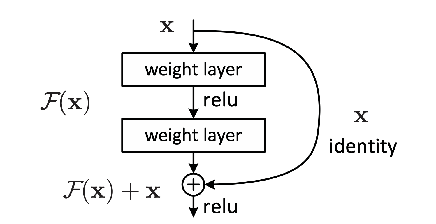
What I realised (me and a number of gruelling Claude sessions) was that the heart of the layer is essentially a single transformation composed of the two matrix multiplications: $48 \to 96$ , and $96 \to 48$ , represented as $W_\text{out} W_\text{in}$ . If you think about it this combined transformation should perform something meaningful for a trained block layer. That is: a random pair should just look like noise since we're chaining two unrelated transformations, while for a trained pair there should be some co-dependency. Or the thought was more like: what if we just plot these?

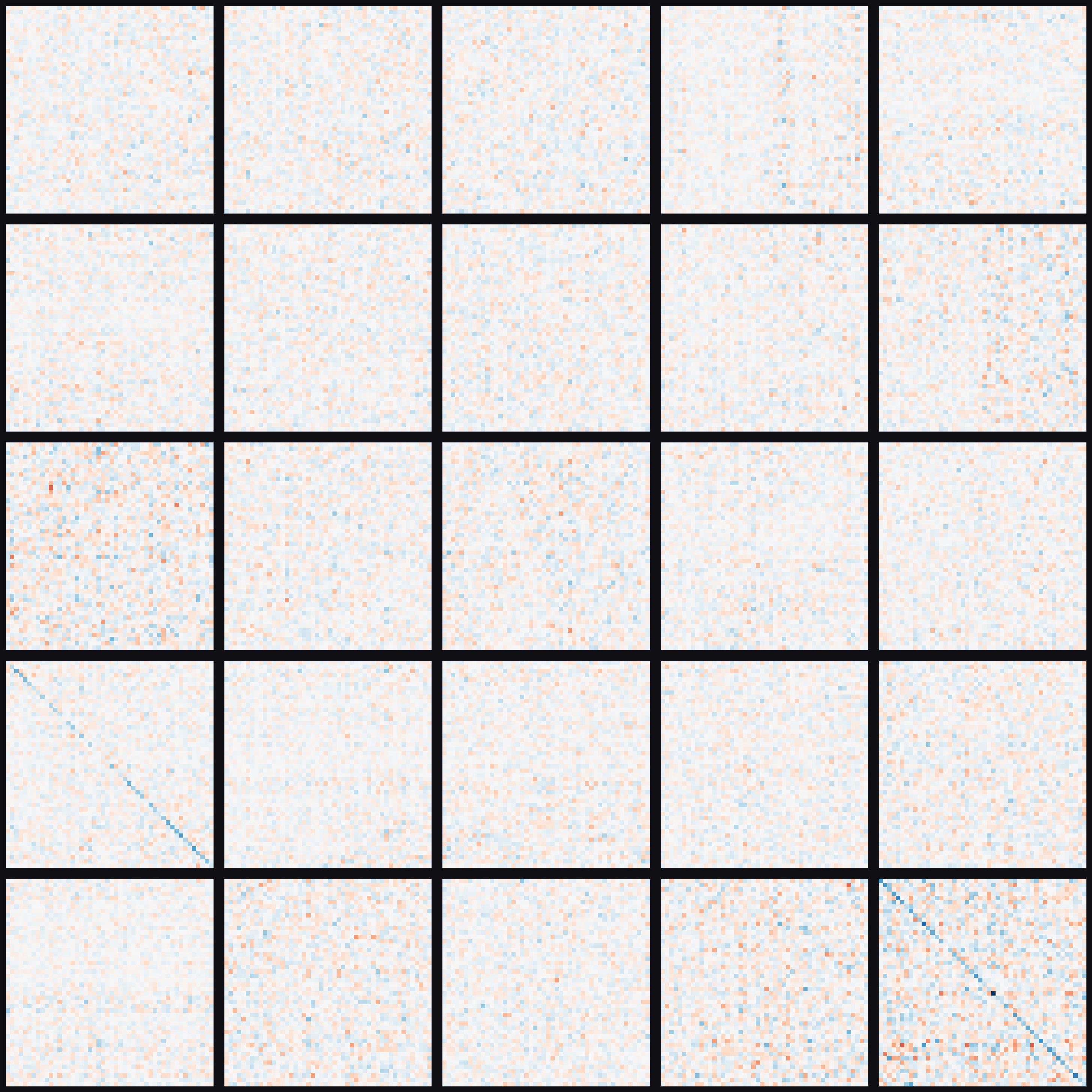
Most matrices do just look like noise here, except for two of them. There's a diagonal pattern that looks to be the same sign. And digging into more pairs via an oracle network it became clear: correct pairs show a strong diagonal signal, while the diagonal of wrong pairs is mostly noise. Since the trace is exactly the sum of diagonal entries, this motivated using $\text{tr}(W_\text{out} W_\text{in})$ as a pairing score. Computing it for all pairs gives us this:

The y axis is here the average trace value over all pairings for each piece, and the x axis is the idx of each pair sorted by trace magnitude. The correct pair stands out at the far right with a strongly negative trace, while the second strongest is still around 0 and far outside any error bounds. The trace measure is a really strong indicator of a correct pair!

Utilizing this together with Hungarian pairing on an oracle network yields 48/48 pairs found! In hindsight I realize we wouldnt even need to optimize for the overall pairing score: the signal is so strong that a greedy pairing would have worked just as well. And also, note that this means we get enough signal from the weight matrices themselves - we don't even have to take into account any of the bias vectors.

With this in mind we can assume we have found the ground truth pair for each block (but we have no way of verifying this yet), and can move on to finding the correct block ordering.

Ordering

The goal was now: given 48 block layers (and a last layer), place them in such an order that the example inputs give identical outputs to the reference predictions (zero error). This is similar to the travelling salesman problem or DNA sequencing, where we need to pick an ordering informed by some cost function. Differences worth noting here are that a cost between two nodes doesn't really make sense here - we need to assemble the full network to produce a valid error value - and edges are directed in the graph, ie we get a different error if we place block A before B, or B before A.

Brute force is of course infeasible. But we can instead try to guide the search via the error signal. You can imagine different simple approaches to search this ordering space: moving a block to another position, moving a chunk of blocks, swapping two blocks, etc, and seeing if the error goes down. Keep the edits that lower the error, and iterate. I tried more sophisticated search methods such as simulated annealing, but in the end the approach I landed on was much simpler, and consisted of three parts:

Greedy initialization. Start with an "empty" network. Pick a block, run the example inputs through it, and calculate the error. Pick the first block as the "single-block" network with the lowest error. For the second block, for each of the remaining 47 blocks insert it before or after the existing block. Calculate the error. Extend the network with the block / placement combo which resulted in the lowest error. And do the same for the remaining blocks until you run out of blocks. This gives a full network that is hopefully relatively close to the solution.
2-opt: For each pair of blocks, swap them and calculate the error. Keep the swap if it lowers the error.
Or-opt: For each block, remove it from the network, and then try inserting it into every other position in the network. Leave it in the position that gave the lowest error.

And this worked! The algorithm in general repeats the 2-opt and or-opt passes until no further improvement is found, but here the correct permutation was found in around 10m in a single greedy -> 2-opt -> or-opt sweep.

Here is an animation showing the solving process with three distinct phases: greedy selection, block swapping (2-opt), and block re-insertion (or-opt). The blue line shows the lowest error achieved so far, and for the last two phases each grey dot is a non-lowest error of an attempted swap. (both the y and x axis have been scaled to make the plot look nicer)

The final order of the weight pieces of the network that achieved zero error is our solution!

That this actually worked means that the error landscape was relatively nice to us, ie it has a "funnel" structure: orderings with lower errors lie closer to the global optimum. So greedy insertion starts us off inside this funnel, and we descend down towards the optimum via swaps. If the loss landscape didn't have this structure this greedy method most likely would not have worked. For instance if there existed several "funnels" for local optima, perhaps as a result of a more complicated network structure.

Intuition

The ordering search works because the error landscape had a nice structure as described above. But why did the trace successfully identify correct weight pairs?

This is not completely clear to me, but here is an attempt at a semi-researched explanation after having dug into the correct network a bit.

The first thing to note is that the gradients of the weight matrices in a block depend on each other. How a gradient update influences $W_\text{in}$ also affects $W_\text{out}$ , and vice versa. That is, the weights co-adapt during training.

Secondly, the trace of the composed weight matrix tells us something about what the transformation does. For $M = W_\text{out} W_\text{in} \in \mathbb{R}^{48 \times 48}$ , the trace equals the sum of its eigenvalues: $\text{tr}(M) = \sum_i \lambda_i$ . Looking at the eigenvalues of $M$ for each correct block, we observe that almost all are negative. Because of the residual structure $\text{block}(\mathbf{x}) \approx (I + M)\mathbf{x}$ a negative eigenvalue of $M$ (and greater than -2) means the effective eigenvalue of $(I + M)$ along that direction has magnitude less than 1, so the block contracts the input toward the origin. In other words, $M$ represents a broadly contractive transformation. The reason this arises is not obvious, but one hypothesis is that it is a result of implicit regularization during training.

So for a correct pair, the fact that $W_\text{out}$ and $W_\text{in}$ have co-adapted to represent a contractive mapping means that the $48 \times 96 = 4608$ elementwise products $W_\text{out}[i,k] \cdot W_\text{in}[k,i]$ that make up the trace are predominantly the same sign. They reinforce each other in the sum, producing a large negative trace.

What about incorrect pairs? For a mismatched pair where $W_\text{out}$ comes from one block and $W_\text{in}$ from another, the contraction structure disappears. $W_\text{out}$ developed its sign pattern in relation to a different $W_\text{in}$ during training. When composed with an unrelated $W_\text{in}$ , the 4608 products have no systematic sign relationship, roughly half positive, half negative, so they cancel in the sum. The trace ends up close to zero because positive and negative terms balance out.

Learnings

Since claude makes writing and running experiments cheap, it's really easy to generate 1000 scripts, lose track of what's been run, what results have been observed, what's still hypotheses and what's actually confirmed - you rack up comprehension debt, and the codebase gradually becomes more and more of a black box. To combat this and to actually make meaningful progress I found it crucial to properly track experiment ideas, plans, results, and the findings and decisions that follow. Importantly to also bridge the amnesia context gap between sessions. In practice:

A single living plan document which details the problem, previous hypotheses, experiments run and their results, interpretation of results and their following consequences, as well as new hypotheses and experiments that are TODO.
Thorough pushback and direction to verify assumptions and explanations about results. I found that you quite easily can come up with plausible explanations and methods which sound good in theory, but which foundations actually crumble when you put them into practice. Something between the LLMs best guess and an overconfident semi hand-wavy explanation to please the user. A constant pressure to focus on first principles and thoroughly verifying assumptions helped overcome these.
Use of several parallel claude code sessions to run independent experiments also helped speed up progress, in tandem with claude's great use of sub agents and running scripts in parallel